Optimal Allocation

We consider the problem of allocating a fixed inventory across multiple locations. To maximize expected sales, units should be distributed so that each site reaches the same sell-through probability. Interestingly, this implies we should often send more units to sites with greater demand uncertainty. We walk through an example that shows how operations teams can apply the strategy in practice.

Maximizing global expected sales

Retailers often place a single large order for a product, then face the challenge of allocating those units across multiple locations. In this post, we consider the optimal number of units to send to each site. We assume the team has already prepared demand estimates for each location – specifically, a distribution $p_i(q)$ representing the probability that location $i$ will sell $q$ units over the season, assuming sufficient inventory.

The key idea is that at the optimal allocation, there are no arbitrage opportunities – that is, you can't improve total sales by shifting a unit from one location to another. If such a transfer could increase net sales, the original allocation wouldn’t be optimal.

To explore this, we start by considering the expected sales at a single location, given that it receives $Q$ units. This is,

$$\begin{array}{c}E(\text{sales at site})={\int }_0^{Q}p(q)\cdot q\cdot dq+Q{\int }_Q^{\infty }p(q)\cdot dq.\end{array}$$

The marginal increase in expected sales (lift in sales given one more unit) is then

$$\begin{array}{c}{\partial }_{Q}E(\text{sales at site})=p(Q)\cdot Q+{\int }_Q^{\infty }p(q)\cdot dq-p(Q)\cdot Q=1-P(d\le Q).\end{array}$$

This is simply the probability of sell-through at $Q$. To eliminate arbitrage opportunities – maximizing global expected sales – units should then be allocated so each site has the same sell-through probability.

Worked example

Suppose you have two locations. In the first site,

$$\begin{array}{c}{\mu }_1=50,{\sigma }_1=10\end{array}$$

In the second site,

$$\begin{array}{c}{\mu }_2=100,{\sigma }_2=50\end{array}$$

Here, $\mu$ and $\sigma$ are the symbols for expected value and standard deviation, respectively. We’ll assume both sales distributions are normal for simplicity. In this case, the probability of sell-through if we send $Q$ units to a site is simply a function of

$$\begin{array}{c}z=\frac{Q-\mu }{\sigma }\end{array}$$

Suppose finally that we have purchased $200$ units total of the product. To find the right amount to send to each location, we’ll assume a common sell-through, set by a common $z$ value. Solving for $Q$ using (5) then gives

$$\begin{gathered} \begin{array}{c}{Q}_1={\mu }_1+{\sigma }_1\cdot z=50+10z \\ \end{array} \end{gathered}$$ $$\begin{array}{c}{Q}_2={\mu }_2+{\sigma }_2\cdot z=100+50z\end{array}$$

From this, we see that each site should first receive units equal to its expected demand. Any remaining inventory is then divided among sites in proportion to their demand uncertainty. When total inventory exceeds overall expected demand, this approach allocates more units to higher-uncertainty sites, allowing you to capture upside if demand spikes there. However, when inventory is below expected demand, the allocation shifts toward lower-uncertainty sites to reduce the risk of unsold stock.

To set $z$, we just need find the value that results in a full allocation of our inventory. Summing (6) and (7), this gives

$$\begin{array}{c}150+60z=200\to z=\frac{5}{6}\end{array}$$

Plugging this into (6) and (7) gives

$$\begin{array}{c}{Q}_1=58\text{ units, }{Q}_2=142\text{ units}\end{array}$$

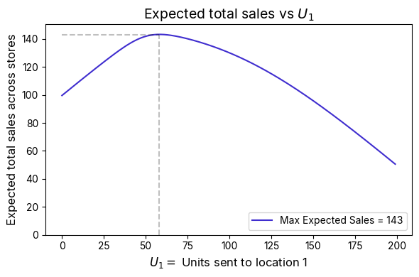
In this case, the total expected sales is around $143$ – just below the total expected sales given unlimited inventory. The figure below plots the total sales across different options for $U_1$.

Figure 1: Total expected sales as a function of $U_1$, the number of units sent to the first location. The remaining $200-U_1$ units are sent to the second location. Around the optimal point, the slope flattens — indicating that total sales are relatively insensitive to small deviations from the optimal split. However, as we push away from this towards the extreme limit of sending all units to just one location (the plot’s right and left extremes), we are limited to that site's expected sales alone.

About VarietyIQ

VarietyIQ helps retailers and brands optimize inventory through smarter forecasting and product curation. We combine advanced data science with domain expertise to improve planning accuracy and unlock growth.

Curious how this analysis might apply to allocation decisions at your business? Get in touch — we’d love to connect.

---

Thanks to Jaireh Tecarro for creating the header image for this post.